The intuition that breaks first
When a training job runs slowly, the instinct is to request more resources. More GPUs means more parallel compute. More parallel compute means faster iteration. That logic is true often enough that it has become default reasoning for most ML teams on shared clusters.
It does not always hold. And it fails in ways that are not obvious until you are already deep into a training run.
The relationship between GPU count and training speed has three distinct regimes. In the first, adding GPUs genuinely accelerates training: throughput increases, wall-clock time falls, and cost-per-epoch drops. In the second, returns diminish: you are adding hardware but spending a growing fraction of each step waiting for coordination, not doing computation. In the third, adding GPUs actively degrades training: convergence slows, results become less consistent, and in some configurations the model fails to converge at all.
Most teams live in regime one for most workloads. Regimes two and three are real, well-documented, and far more common than benchmarks suggest, because benchmarks are designed by people who know how to avoid them.
This article explains why regimes two and three exist, what causes them, and what to do about it.
Start with Amdahl's law, then go further
The classic framework for parallel scaling is Amdahl's law. It says the maximum speedup from parallelization is limited by the fraction of work that cannot be parallelized. If 10% of your training step is inherently serial, no amount of GPU scaling will exceed a 10x speedup, no matter how many devices you add.
But there is a part of the story Amdahl's law does not capture: the serial fraction grows as you add more GPUs.
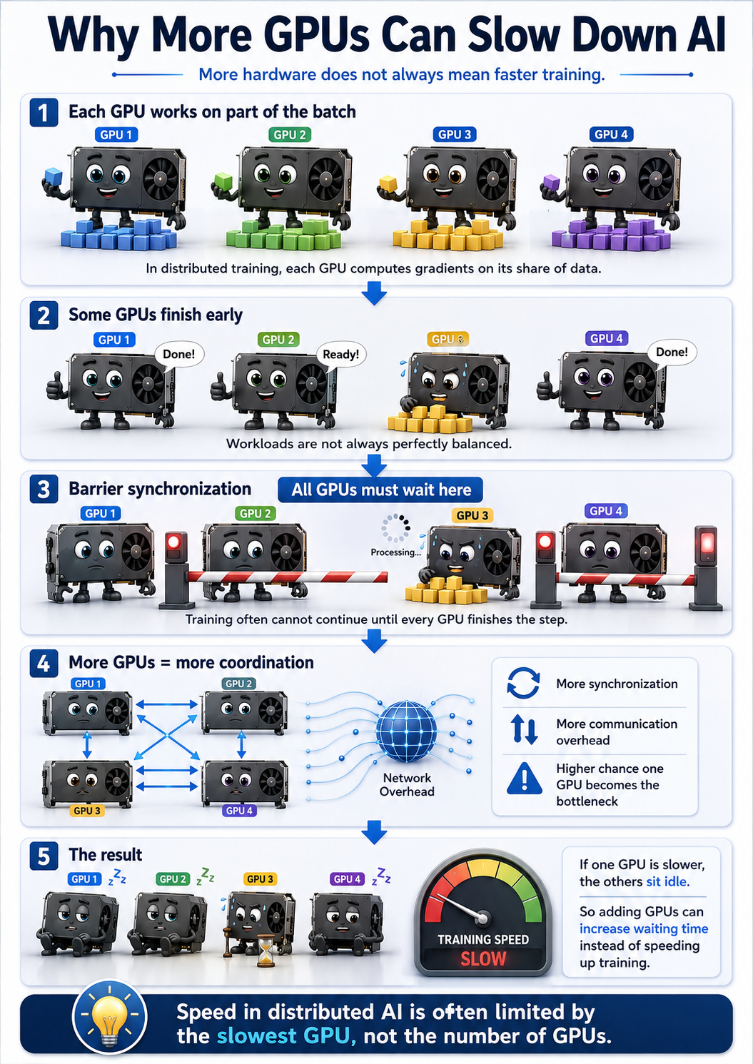
In distributed training, after every backward pass, all GPUs must agree on the gradient update before taking the next step. This coordination step, called an all-reduce, requires every GPU to send its gradients to every other GPU and combine them. The more GPUs you have, the more data needs to move, and the longer this coordination takes.
Consider a concrete example. A model with 100 million parameters sends 400 MB of gradient data per all-reduce step. On two GPUs connected over NVLink (the fast GPU-to-GPU interconnect inside a single server), that exchange takes about 1 to 2 milliseconds. On 256 GPUs spread across multiple nodes connected by InfiniBand, the same exchange can take 50 to 100 milliseconds, depending on network load, switch configuration, and what other jobs are running on the same cluster.
If your actual compute step takes 200 ms and all-reduce adds 50 ms, you are spending 25% of every training iteration just waiting for GPUs to talk to each other. That overhead applies to every step, across every epoch, for the entire run. It does not show up in single-GPU benchmarks. It is invisible until you scale.
You paid for 256 GPUs. You got the effective throughput of maybe 80, once communication cost is properly accounted.
The math problem hiding inside every gradient update
Beyond communication time, there is a subtler issue: the result of a distributed training step depends mathematically on how many GPUs participated.
This sounds strange. The same model, the same data, the same loss function — how can the answer depend on GPU count?
It comes down to a property of floating-point arithmetic. On a computer, addition is not perfectly associative. That means (a + b) + c does not always equal a + (b + c) when numbers are represented in finite precision. The difference is usually tiny, but it is nonzero.
A gradient reduction across multiple GPUs is, at its core, a very large sum: all the gradient values from all the parameters, combined across all the devices. With 2 GPUs, the sum happens in one order. With 8 GPUs, the ring topology changes and the sum happens in a different order. With 64 GPUs, a tree reduction algorithm picks yet another order.
Each ordering produces a slightly different result. On its own, any one difference is negligible. But gradient descent runs for tens of thousands of steps. Small numerical differences in each gradient update accumulate over time. The path the optimizer takes through the loss landscape shifts. The solution the model converges to can change, sometimes in ways that matter for scientific validity, not just benchmark scores.
This is not a bug in any particular library. It is a consequence of how floating-point arithmetic works, and it is not something you can fix by setting a random seed.
What happens when you change GPU generations
The problem compounds when the hardware itself changes, which often happens naturally as teams scale from development clusters to production allocations.
Different GPU generations handle floating-point arithmetic differently by default. Newer architectures frequently introduce precision modes that trade numerical fidelity for higher throughput. A training script that ran at full 32-bit precision on one generation may silently run at a reduced precision mode on the next, without any code change and without any warning in the logs.
| Scaling scenario | What changes | Visible in logs? |
|---|---|---|
| 2 GPUs to 8 GPUs, same hardware | Reduction order, ring topology | No |
| Same GPU count, newer hardware generation | Default precision mode, cuDNN algorithm selection | No |
| Both: more GPUs and newer hardware | Precision, reduction order, network topology, NCCL algorithm | No |
| Different cluster, same job script | Network bandwidth, contention, node placement | No |
None of these changes require a code modification. All of them can alter numerical behavior. When a team moves from a small development allocation to a large production run and observes different training dynamics, the instinct is to look for a bug. There is usually no bug. Several numerical properties changed simultaneously, each small in isolation and collectively significant.
Scaling up GPU count and changing hardware generation at the same time is particularly risky because the effects interact. The gradient reduction order changes with GPU count. The precision mode changes with the hardware generation. The NCCL communication algorithm changes with both. A training run that was validated on a smaller, older allocation is not guaranteed to reproduce on a larger, newer one, even with the same code, the same data, and the same random seeds.
The slowest GPU sets the pace for everyone
There is a third mechanism that is rarely discussed in introductory distributed training resources: barrier synchronization.
In standard synchronous training, all GPUs must finish their backward pass before the gradient reduction can begin. This is enforced by a synchronization barrier: every GPU waits until every other GPU has arrived.
On a perfectly homogeneous cluster with identical hardware, identical temperatures, and no competing jobs, every GPU arrives at the barrier at roughly the same time. The wait is negligible.
On a real HPC cluster, that assumption does not hold. Different nodes experience different memory pressure from co-located jobs. Different GPUs in the same chassis run at different temperatures depending on their position in the airflow. Different network paths between nodes have different latencies depending on what else is running on the same switch fabric.
The speed of the entire distributed job is bounded by the slowest GPU in every step. If 63 GPUs finish their backward pass in 180 ms and one GPU takes 240 ms because it is thermally throttled, all 63 faster GPUs wait 60 ms at the barrier. Every step. Across 100,000 training steps, that adds up to roughly 100 hours of wasted compute time, invisible in any single-step measurement but cumulatively devastating.
This effect gets worse as GPU count grows. The probability that at least one GPU is slow in any given step increases with job size. With 2 GPUs the chance is low. With 256 GPUs, across a long run, it is nearly certain. The more GPUs you add, the more time every other GPU spends waiting at barriers.
This is why straggler mitigation strategies, asynchronous gradient updates, and load-aware job placement tools exist. They are not theoretical features. They are responses to a real and measured problem in production distributed training on shared clusters.
Why scientific workloads are hit harder
Everything above applies to standard deep learning. For scientific ML, meaning models trained against physical laws, simulations, or domain-specific ground truth, the consequences are more serious because the failure mode changes.
A standard image classification model that converges differently due to floating-point reduction order produces a model that classifies images slightly less accurately. The failure is visible and measurable.
A physics-informed neural network that converges to a solution violating the governing equations produces numbers that look like predictions. Those numbers pass loss thresholds. They appear in output files. They may even look reasonable on casual inspection. But they do not satisfy the physical constraints the model was supposed to enforce. The failure is invisible unless you run domain-specific validation.
In scientific contexts, adding more GPUs can change what the model learns in ways that matter scientifically, not just what score it gets on a benchmark. That is a qualitatively different kind of risk than slower convergence.
Three questions before you scale
The right question before requesting a large GPU allocation is not "how many GPUs do I need?" It is "does my workload actually benefit from more GPUs?"
Three properties determine the answer.
Is the workload compute-bound or communication-bound? If your model spends most of its time doing matrix multiplications, adding GPUs helps because you can split that work. If your model has many small operations requiring frequent inter-GPU communication, as graph neural networks often do, adding GPUs may add more communication overhead than compute throughput.
Is the training numerically stable under different GPU counts? This is not something you can determine by inspection. It requires running the same configuration at different scales and comparing results, not just accuracy metrics, but whatever scientific validity metric actually matters for your application.
Does your cluster have the network bandwidth to support the communication volume you are generating? On a shared HPC cluster, this is not guaranteed. A job that ran well on a lightly loaded cluster may run significantly worse on a busy one. The job specification did not change. The effective network bandwidth did.
A simple protocol worth running before every large job
The most useful practice before committing to a large distributed training run is a scaling efficiency measurement. The protocol takes a few hours and can save days or weeks of wasted allocation.
Train for a fixed number of steps, a few hundred is usually enough, at 1, 2, 4, and 8 GPUs. Measure wall-clock time per step, not total throughput. Plot the actual speedup ratio against the theoretical ideal. Find where the curve starts bending away from linear.
If your speedup at 4 GPUs is 2.5x instead of 4x, you are already in regime two. Extrapolating to 32 or 64 GPUs based on that trajectory will land you firmly in regime three.
For scientific workloads, add one more check: compare your domain validation metric at each scale point. If physics residuals, conservation law errors, or application-specific accuracy degrade as GPU count increases, you have found the numerical stability ceiling for your workload. Running beyond it produces results that are fast to compute and wrong to use.
The compute cost of this protocol is small. The information it gives you is the most important input to a scaling decision. It is almost never done in practice.
The practical takeaway
GPU count is not a proxy for training quality. It is an infrastructure parameter with complex effects on communication overhead, floating-point behavior, synchronization cost, and for scientific workloads, result validity.
The teams doing the best work on HPC clusters are not the ones running the largest jobs. They are the ones who know their workload's scaling behavior, have identified the scale ceiling, and design their experiments to stay inside it.
Adding GPUs is a one-line change to a job script. Understanding what that change actually does to your training is the engineering work.
References
- Amdahl, G. M. (1967). Validity of the single processor approach to achieving large scale computing capabilities. Proceedings of AFIPS Spring Joint Computer Conference, 483–485.
- Recht, B., Re, C., Wright, S., & Niu, F. (2011). Hogwild!: A lock-free approach to parallelizing stochastic gradient descent. NeurIPS, 24.
- Sergeev, A., & Del Balso, M. (2018). Horovod: Fast and easy distributed deep learning in TensorFlow. arXiv:1802.05795. Available: arxiv.org/abs/1802.05795
- Bouthillier, X., et al. (2021). Accounting for variance in machine learning benchmarks. MLSys, 3. Available: arxiv.org/abs/2103.03673
- NVIDIA Corporation. (2023). cuDNN Developer Guide. Documents runtime algorithm selection behavior and determinism opt-in requirements. Available: docs.nvidia.com/deeplearning/cudnn/developer-guide/
- PyTorch Team. (2024). Reproducibility. PyTorch Documentation. Available: pytorch.org/docs/stable/notes/randomness.html